


RSL III NX
One-dimensional local seismic response analysis in the browser — propagate an accelerogram from bedrock to the surface through your soil column with the equivalent-linear method, and get response spectra, amplification and the ICMS microzonation factors, aligned with NTC 2018 and Eurocode 8.
What it does
RSL III NX takes a stratigraphic column and a bedrock accelerogram and returns the seismic motion at the surface — response spectra, amplification and the ICMS Level-3 microzonation factors — through an iterative equivalent-linear analysis, entirely in the browser.
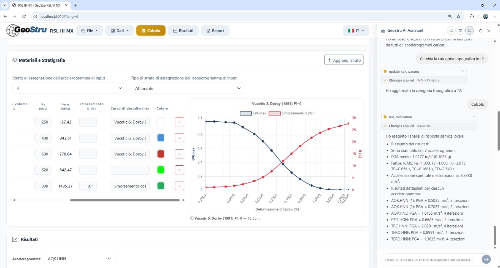
Layered soil model — each layer by unit weight, small-strain shear-wave velocity Vs, damping and the degradation curves G/Gmax-γ and ξ-γ (Vucetic-Dobry, Seed-Idriss, Darendeli and custom).
Equivalent-linear analysis — an iterative scheme that converges on the effective shear strain, capturing the soil's nonlinear stiffness and damping.
Flexible input motion — imported accelerograms (PEER, ITACA, ESM, CSV), synthetically generated signals or built-in example records at bedrock.
Complete outputs — surface PGA, response spectra Sa(T), Sv(T) and Sd(T), the frequency amplification function, elastic and design spectra and the ICMS 2018 factors.
Seismic parameters built in — ag, F0 and Tc* from coordinates or address for every limit state (SLO, SLD, SLV, SLC).
Report-ready deliverables — Word reports for seismic microzonation and site-response studies.
The equivalent-linear method
The equivalent-linear method approximates the soil's nonlinear behaviour with a sequence of linear analyses, updating stiffness and damping until they match the strain the shaking actually produces.
Layer discretisation — the column is split into thin sub-layers and the transfer function H(ω) is built from the plane-wave coefficients between base and surface.
Effective shear strain — each iteration takes the effective strain as γeff = 0.65 · γmax and reads the secant shear modulus and damping from the degradation curves.
Convergence — stiffness and damping are updated and the analysis repeats until the strain change is small — typically 4–8 iterations; many more points to a strongly nonlinear regime.
Soil column and dynamic curves
The reliability of a 1D analysis rests on the soil column and the curves that describe how each layer softens with strain.
Layer parameters — thickness, unit weight ρ, small-strain velocity Vs and the maximum shear modulus Gmax = ρ · Vs², with a baseline damping ξmin.
Degradation curves — G/Gmax-γ and ξ-γ from established models — Vucetic-Dobry (1991) for clays by plasticity index, Seed-Idriss (1970) for sands, Darendeli (2001) — or your own tabular data.
Bedrock — the deepest layer is the seismic bedrock (Vs ≥ 800 m/s), so the 1D wave propagation is anchored to a rigid base.
Input motion
The analysis is driven by the reference accelerogram at bedrock and by how you combine the records.
Real records — import accelerograms in PEER, ITACA, ESM or CSV format; the app reads the time step Δt and the duration automatically.
Synthetic signals — generate spectro-compatible motions by band-pass FFT filtering with a seismic envelope, or start from the built-in example records.
Analysis type — single site and record, multi-input (several accelerograms averaged per NTC 2018) or multi-site comparison of stratigraphies.
Code guidance — NTC 2018 asks for at least seven spectro-compatible accelerograms; prepare and scale them in GeoStru Spectra or REXEL, as RSL III does not rescale automatically.
How it works
A guided flow takes you from the soil column to an exported report in seven steps.
1 · Stratigraphy — define each layer's thickness, Vs, density and damping and pick its degradation curves; close the column on bedrock (Vs ≥ 800 m/s).
2 · Dynamic curves — assign the G/Gmax and damping curves per layer, from the library or from your own data.
3 · Input accelerogram — load the bedrock motion (PEER, ITACA or CSV); the time step and duration are detected automatically.
4 · Analysis type — single-site, multi-input or multi-site.
5 · Equivalent-linear computation — the app builds the transfer function, estimates γeff = 0.65 · γmax and iterates the stiffness and damping to convergence.
6 · Results — the response spectrum against the NTC 2018 reference, the input/output Fourier spectra, the γmax(z), amax(z) and τmax(z) profiles and the ICMS amplification factors.
7 · Export — a Word report for the microzonation or site-response study.
Inputs and outputs
What you enter
Soil column — layer thickness, unit weight, Vs and damping, with the degradation curves.
Input motion — the bedrock accelerogram(s), imported or synthetic.
Site — coordinates or address, so ag, F0 and Tc* are retrieved for every limit state.
What you get
Response spectra — Sa(T), Sv(T) and Sd(T) at the surface, against the NTC 2018 reference.
Amplification — the frequency transfer function and the ICMS 2018 factors (FA, FH, FT).
Depth profiles — the maximum shear strain γmax(z), acceleration amax(z) and shear stress τmax(z).
Deliverables — a Word report for microzonation and site-response studies.
Who it's for
Geologists · Geotechnical and seismic engineers · Consulting firms. RSL III NX is for anyone who runs site-specific ground-response analyses — for seismic microzonation, building design on soft soils and seismic hazard assessment — and wants a single web tool that goes from the soil column and the bedrock motion to code-ready surface spectra and amplification factors.
Why it's different
Runs directly in the browser — no installation, always up to date.
A full equivalent-linear 1D analysis with the standard degradation-curve library built in.
Real, synthetic and multi-record input motions, with single-site, multi-input and multi-site analyses.
Surface spectra, the amplification function and the ICMS 2018 factors in one place.
Seismic hazard parameters (ag, F0, Tc*) retrieved automatically for every limit state.
Word reports ready for a Level-3 seismic microzonation study.
Frequently asked questions
What does "equivalent-linear" mean?
It approximates the soil's nonlinear response with a sequence of linear analyses, updating stiffness and damping at each iteration until they match the strain the shaking produces.
Where do the Vs velocities come from?
From direct seismic measurements — MASW, ReMi, cross-hole, down-hole or SCPT; empirical SPT correlations are too uncertain for a reliable analysis.
How deep should the column go?
Down to the seismic bedrock (Vs ≥ 800 m/s), typically between 5 and 300 m in Italy.
How many accelerograms do I need?
NTC 2018 asks for at least seven spectro-compatible records; RSL III does not rescale them, so prepare them in GeoStru Spectra or REXEL.
Which amplification factor should I use?
FA for low-rise buildings, FH for mid-rise, and the full spectrum for tall structures.
Does it compute post-seismic settlements?
No. RSL III covers ground response; for liquefaction and settlements use LiquiTer NX.
Ready to start with RSL III NX?
Choose your plan and start using RSL III NX today. Runs in the browser, always up to date, no installation required.